How-To
This tutorial shows how to use VG in an ipython shell. The data used for the examples is provided in the sample.met file. Everything here should work without any changes to the config_template.py file.
Another tutorial shows how to configure VG to use other data.
Initialization
In [1]: from varwg import VarWG

In [2]: my_vg = VarWG(("theta", "Qsw", "ILWR", "rh", "u", "v"))
Loading input data.
Reading /home/docs/checkouts/readthedocs.org/user_builds/vg-doc/envs/latest/lib/python3.13/site-packages/varwg/sample.met
	Found 0 missing or nan values
Fitting seasonal distributions.
	Fitting SlidingDist(normal) to theta

	Fitting KDE to Qsw

	Fitting SlidingDist(normal) to ILWR

	Fitting SlidingDist(truncatednormal) to rh

	Fitting KDE to u

	Fitting KDE to v
Initialization involves converting the input to stationary, standard- normal distributed variables via day-of-year-specific quantile-quantile transform. As this is time-consuming, the fitting results are cached on the hard-drive (in the conf.cache_dir to be exact).
More information on all the initialization parameters: varwg.VarWG.__init__().
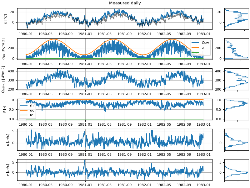
The varwg.VarWG class provides a number of methods for plotting various results. To see the input time series one can use varwg.VarWG.plot_timehists():
In [3]: figs, axes = my_vg.plot_meteogram_daily(figsize=(8, 6))
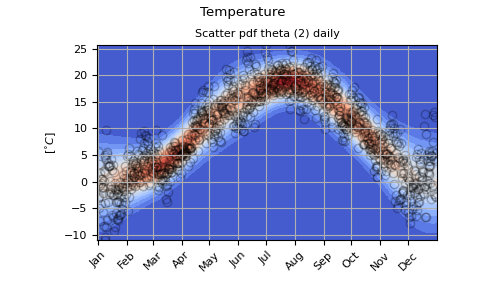
The fitting of the daily seasonal distribution can be visualized with varwg.VarWG.plot_daily_fit():
# the plot_quantiles and plot_fourier parameters can be omitted in order to
# get more information on the fitting.
In [4]: my_vg.plot_daily_fit("theta", plot_quantiles=False, plot_fourier=False)
Out[4]:
([<Figure size 485.41x300 with 1 Axes>],
 [<Axes: title={'center': 'Scatter pdf theta (2) daily'}, ylabel='[$^{\\circ}C$]'>])

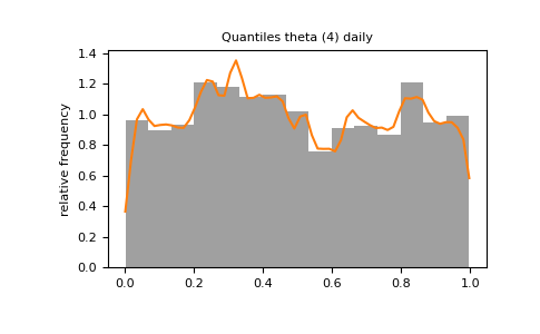
# if the fit is good, the histogram of the quantiles should be roughly
# uniformly distributed
In [5]: my_vg.plot_daily_fit("theta", plot_fourier=False)
Out[5]:
([<Figure size 485.41x300 with 1 Axes>, <Figure size 485.41x300 with 1 Axes>],
 [<Axes: title={'center': 'Scatter pdf theta (3) daily'}, ylabel='[$^{\\circ}C$]'>])
If you are not satisfied with the conversion, adjust the settings in config.py and initialize VG again with the refit-parameter:
In [6]: my_vg = VarWG(("theta", "Qsw", "ILWR", "rh", "u", "v"), refit="ILWR", verbose=False)

# you can also supply multiple variables to refit
In [7]: my_vg = VarWG(("theta", "Qsw", "ILWR", "rh", "u", "v"), refit=("ILWR", "rh"), verbose=False)
Fitting
Calling varwg.VarWG.fit() fits the stochastic process to the transformed data. When called without parameters, an order selection is performed to find a good compromise between the fit and the number of parameters. Per default, the moving average part is neglected (q=0).
In [8]: my_vg.fit()

# the autoregressive order can be fixed like this
In [9]: my_vg.fit(3)
Simulation
Without parameters, varwg.VarWG.simulate() generates time series similar to the input data.
In [10]: times_out, sim_data = my_vg.simulate()
The output is also stored in the out_dir (specified in config.py) as text file.
At this point it can be assessed whether the order selection was successful. varwg.VarWG.plot_autocorr() provides a shortcut to plot the autocorrelations of residuals, measured (continuous line) and simulated (dashed line) data (in the “real” and the “transformed” domain)
# in a real ipython shell one call to plot_autocorr suffices. here i have
# to hack to get all figures
In [11]: figs = my_vg.plot_autocorr()

In [12]: varwg.plt.figure(5)
---------------------------------------------------------------------------
NameError                                 Traceback (most recent call last)
Cell In[12], line 1
----> 1 varwg.plt.figure(5)

NameError: name 'varwg' is not defined
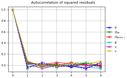
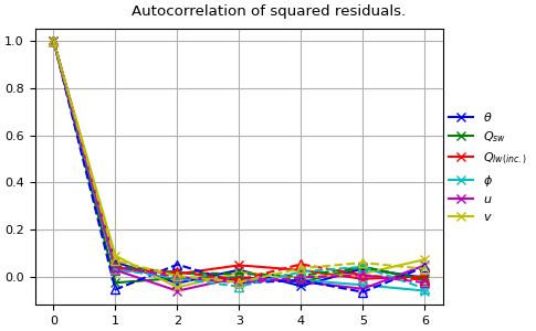
Would the fit have been less good, one could consider calling varwg.VarWG.fit() again with a higher p.
Scenarios
Scenarios are implemented through changes based on the primary variable (default: air temperature). The primary variable can be specified by the parameter primary_var in varwg.VarWG.simulate().
Increased mean (theta_incr)
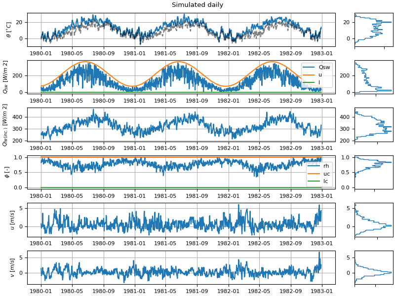
In [13]: times_out, sim_data = my_vg.simulate(theta_incr=4)

# we can display the result like we did above with the input data
In [14]: figs, axes = my_vg.plot_meteogram_daily()
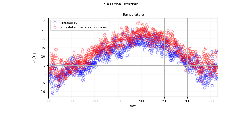
Another way to visualize the simulation is offered by the method varwg.VarWG.plot_doy_scatter():
In [15]: my_vg.plot_doy_scatter("theta", figsize=(8, 4))
Out[15]:
(<Figure size 800x400 with 1 Axes>,
 <Axes: title={'center': 'Temperature'}, xlabel='doy', ylabel='$\\theta$ [$^{\\circ}C$]'>)
Increased variability via enhanced episodes (mean_arrival and disturbance_std)
For increased variability, a Poisson-process is used to set the theoretical mean of the autoregressive process. Durations of episodes are drawn from an exponential distribution with the mean specified as mean_arrival. For each episode, a disturbance is drawn from a normal distribution with the standard deviation of disturbance_std.
In [16]: times_out, sim_data = my_vg.simulate(mean_arrival=7, disturbance_std=4)
Providing a climate signal (climate_signal)
VG can be made to follow a specific signal by passing an array with the climate_signal parameter.
Output
varwg.VarWG.simulate() dumps the generated time series in the out_dir (specified in config.py) as an ascii file. The filename is chosen by the fitting parameters (Example: VARMA_p3_q0_sim.dat)
Disaggregation
See varwg.VarWG.disaggregate()
In [17]: times_dis, sim_dis = my_vg.disaggregate(("Qsw", "u", "v"))
Disaggregation also regenerates the seasonal changes in daily cycle.
In [18]: fig, axes = my_vg.plot_daily_cycles("Qsw")
---------------------------------------------------------------------------
NameError                                 Traceback (most recent call last)
Cell In[18], line 1
----> 1 fig, axes = my_vg.plot_daily_cycles("Qsw")

File ~/checkouts/readthedocs.org/user_builds/vg-doc/envs/latest/lib/python3.13/site-packages/varwg/core/plotting.py:1816, in Plotting.plot_daily_cycles(self, var_names, rain_thresh, **fig_kw)
   1812     rain_comparison = True
   1814 figs, axes = [], []
   1815 month_iis = [
-> 1816     varwg.times.time_part(self.times_orig, "%m") == month
   1817     for month in range(1, 13)
   1818 ]
   1819 hour_iis = [
   1820     varwg.times.time_part(self.times_orig, "%H") == hour
   1821     for hour in range(24)
   1822 ]
   1823 month_sim_iis = [
   1824     varwg.times.time_part(self.dis_times, "%m") == month
   1825     for month in range(1, 13)
   1826 ]

NameError: name 'varwg' is not defined
Tips
Caching: Once you change anything in the met_file you have to empty the cache! To empty the cache, simply delete everything in the
cache_dir(specified inconfig.py) or call the functionvarwg.delete_cache()